A technical career retrospective part 7
IBM MVS: 1984 - 1985
Why this post?
The time frame of this post and the previous two posts all overlap.
A short-term project pulled me in due to my Fortran knowledge.
TL;DR
My initial encounter with the IBM mainframe environment.
Disclaimer
My practical experience with the IBM series of mainframes spanned about 10 years, but this is where it started.
Yep, once again take every detail I write here with a large bucket of salt! Some of it I’m more confident than others - but I could simply be more confidently wrong. I’ve checked what I could, but there’s a lot here that is more of my impressions of the situation and not documented facts. There are some topics that I’m greatly simplifying - this isn’t intended to be reference material, just identifying some highlights of what stood out to me at the time.
My introduction to MVS
Having previously demonstrated my skills with Fortran on GCOS, I was assigned to work on a Fortran project on an IBM system. This was primarily intended to be an interactive task, and expected to be completed in a very short timeframe.
But first, I needed to learn enough about MVS to do the work.
Unfortunately, the individual I was working with on this project was also an IBM novice. Neither one of us had the background or training to be particularly effective doing this, but we would do our best.
IBM uses different terminology than Honeywell (and others). What the whole world (other than IBM) calls a “file”, IBM refers to as a “dataset”, and what everyone else calls a “disk drive”, IBM refers to as a “Direct Access Storage Device”, or DASD. What we call RAM or memory, IBM calls “main storage”. (And the list goes on.)
This made it difficult to read and understand the documentation that was available to us, and almost impossible to find certain information because we didn’t know the terms to look for in the indexes.
What was different about IBM MVS?
Data management. The one feature that most impressed me about the environment was how focused MVS is on managing and optimizing the use of data in a production data-processing environment.
Datasets (files)
I’m not even sure where to start with this. There are so many items to mention. Working with datasets in the IBM world was fundamentally different than everywhere else.
Dataset names
Dataset names are a maximum of 44 character. A name is generally composed of two or more qualifiers, separated by periods. Each qualifier is 1-8 characters in length. The first qualifier is usually either a username or a system name. This first qualifier is commonly referred to as the “High-level qualifier” (HLQ).
When the HLQ is the user, the most common convention for the second qualifier is to identify the system being worked on, and the third qualifier generally indicates the type of dataset.
For example, if my username is KWW, and I’m working on the inventory system, and I have a dataset containing cobol code, I might be using a dataset name like KWW.INVENTRY.COBOL, and the JCL that I’m using with it might be in KWW.INVENTRY.JCL. Those would be the datasets I’m using in development. The production system would more likely have names PROD.INVENTRY.MASTER.DATA or PROD.INVENTRY.PGM.LIB
Dataset catalogs
The file system is “flat” - there is no concept of a directory structure, at least not in the same way that there is in a Linux or Windows file system. Instead, MVS tracks datasets in two different ways.
Every DASD Volume (a.k.a “hard drive”) has a Volume Table Of Contents (VTOC). A dataset can be accessed by referencing the dataset name and the volume on which it’s stored. Additionally, MVS stores dataset location in a catalog.
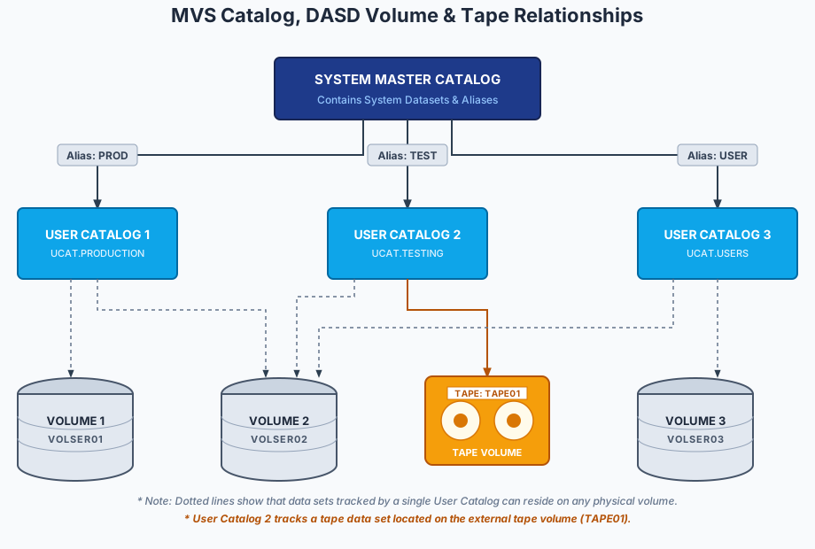
There is a System Master Catalog that contains the information for critical system files needed for the system to start. It also contains the references to the User Catalogs, which are used to store the information for all other datasets. The master catalog also stores the alias entries that map each HLQ to a user catalog that will store the entries for that HLQ.
Accessing a dataset like KWW.INVENTRY.JCL without specifying a volume label means that MVS will first find the HLQ (KWW) in the master catalog to find the proper user catalog. That user catalog would then be searched for that dataset name. When found, the catalog entry contains the volume. MVS would then read the VTOC for the volume to find the specific location of that dataset.
What surprised me most about catalogs is that a User Catalog entry doesn’t need to reference a DASD volume. MVS supported both tape reels and other types of storage devices as “first-class citizens” of the storage environment.
An output tape can be assigned a dataset name and cataloged, at which point the catalog entry is made with the dataset name and the tape label name.
Allocating that dataset at a later time issues a tape mount request to the operator. This allows the developer to not need to know what physical tapes are used to store their data - and to a large extent, not even know whether the data is on tape or disk.
Dataset types
Not all datasets are the same. There are fundamentally different types based upon how they are structured and used.
Fixed Block
The “standard” type of dataset is known as a Fixed Block (FB) file. It is a sequential file where every record is the same length. This comes as a direct result of the old punch card standard, where everything was read or written as 80-column cards.
Most datasets used for development would use an FB 80 format. This includes the source code, jcl, and even compiled code.
Program data would frequently also use an FB format, but the length may vary based upon the requirements of the system. (When the systems were more punch-card oriented, they would still be built around the 80-column format, but programmed to potentially require more than one card per data record.)
With every record being the same size, it is possible to modify FB datasets in place. A record can be read, updated and written back to the file.
Variable Block
MVS also supports a Variable Block (VB) format. In a VB dataset, a 4-byte record length is stored at the beginning of each record. These files cannot be modified in place if the length of a record is being changed.
Partitioned Datasets (PDS)
A Partitioned Dataset (PDS) serves as a “container” for multiple files, known as “members”. PDSs are used extensively in the operating system and in software development as libraries for related stuff.
For example, a system may have many JCL streams for different functions, or the source code may be broken down into different compilation units.
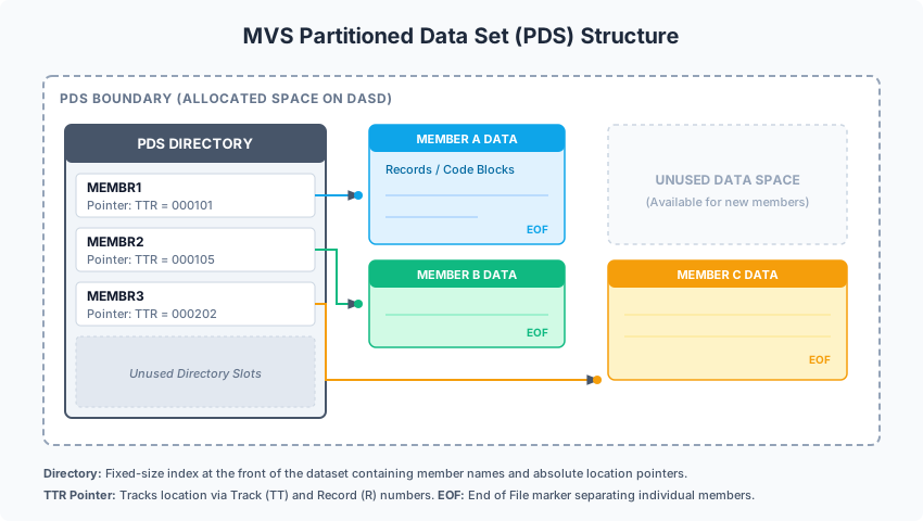
These members are identified by a 1-8 character name enclosed in parens as part of the dataset name.
What I identified as the dataset KWW.INVENTRY.JCL would more likely be a PDS with members like KWW.INVENTRY.JCL(DAILY), KWW.INVENTRY.JCL(WEEKLY), KWW.INVENTRY.JCL(MONTHLY), KWW.INVENTRY.JCL(REPORTS), etc.
This same type of structure would be used for your source code modules and other components being developed for a system such as documentation files.
PDSs had the limitation that members would not be edited in place. Every time a member was edited and saved, it would be appended to the end of the dataset. If there was not enough free space remaining at the end of the dataset, the operation would fail. A utility would then be run to condense the PDS to reclaim the previously-wasted space. This failure mode made PDSs not particularly suited for storing data.
Generation Data Group (GDG)
A common pattern for maintaining data was not to update data in place, but to write a new dataset with the changes having been applied to it. (This was necessary for punch cards and magnetic tape processing, and useful for DASD-based processing.)
A program would read an “old” file along with an “update” file, process the updates, and write the modified records to a “new” file. When working with tape, this pattern provides a roll-back feature, as the “old” file remains available until the tape is recycled.
A GDG facilitates this in a DASD environemnt by managing a dataset name and supplying a numeric suffix identifying the generation of that dataset.
Instead of a single dataset named PROD.INVENTRY.MASTER.DATA, it would be more common to define it as a GDG. The dataset name wouldn’t change, but the actual file stored on disk would have a name like PROD.INVENTRY.MASTER.DATA.G0001V00. (The suffix was commonly referred to as the “goovoo” number.)
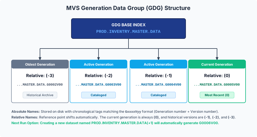
A GDG would be defined as keeping some fixed number of generations, automatically rolling off the oldest when a new one is created.
When accessing a GDG in JCL, a relative generation number would be used. This generation number is specified in parens after the base name. Specifying PROD.INVENTRY.MASTER.DATA(0) is referring to the most recent file, PROD.INVENTRY.MASTER.DATA(1) would be the new file being created, and PROD.INVENTRY.MASTER.DATA(-1) is a reference to the generation before the current.
This allowed JCL to be written that doesn’t need to change. The typical processing pattern reads the (0) and writes the (1). Delete the (0) to roll back because of a program or data problem.
Generate a summary report of changes by running a comparison between (-1) and (0)
Summary
The features shown here are still available in modern IBM z/OS mainframe environments, even though the rise in database usage has reduced their importance.
Footnotes
MVS is alive and well in the retrocomputing world. The Hercules emulator with the “MVS Turnkey system 5” makes it very easy to get your own MVS 3.8 system up and running.
Finally, the project I mentioned at the top? It was scrapped after a month or so of work. The requesting user discovered that a spreadsheet was easier to use and sufficient for their purpose.