A technical career retrospective part 10

Why this post?

I was hired by the Monumental Life Insurance Company in June 1986 in their programming department. My first exposure to a real batch-oriented production system environment!

I covered some MVS fundamentals back in part 7 from a user-facing perspective.

The management of datasets in MVS was unique to me. I have never worked on any other platform that required so much specific technical knowledge when working with data being stored on hard drives. Every other system I’ve used had completely abstracted away the physical geometry, making it invisible to the application developer.

TL;DR

I learned a lot more about MVS this time around, giving me an even deeper understanding of the mainframe environment.

Disclaimer

IBM z/OS is still currently a very active system. It has also made tremendous advancements in the past 40+ years. A lot of what I describe here may have been true in 1986 but isn’t true anymore. Don’t take what I say about “MVS - then” to be relevent when talking about “z/OS - today”.

Overview

My job revolved around one small part of the large system that effectively ran the company. During the day, people working in various departments would enter data. At night, that data would be processed as updates and applied to the master files. Various reports and extracts would be created. Reports and extracts would be created from them. Reports would be printed and distributed.

At times, and for various reasons, the programs running at night would crash and need to be fixed that same night.

The nature of the fixes would vary. In some cases, a dataset couldn’t be allocated or ran out of space. In some cases, the update was flawed and would be removed. In others, a program might need to be fixed.

In either case, it was considered urgent and the work needed to be done for the nightly cycle to complete on time.

Being “on call” for a day, or week, was considered normal and expected. You got used to getting calls at 2 AM letting you know about a problem - and then waking up enough to take care of them. That was just part of being a mainframe programmer in the 70’s and 80’s.

Due to the full-screen nature of the IBM 3270 terminals, a special terminal was needed for remote connectivity. We used the Informer brand of terminals. Anyone being On Call would sign one out to take home.

Because of my on-line activities at that time, I already had a second phone line available to me. I was one of the few people who could log on and research a problem and still be on the phone with either the operators or co-workers.

One non-programming factor in ensuring a successful nightly cycle is managing DASD and datasets. I spent a lot of time gaining an understanding of the datasets being used at different parts of the cycle.

DASD allocation

Block size

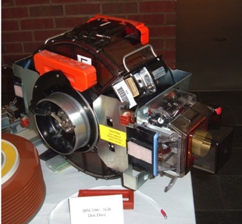
The first truly eye-opening issue I learned was the importance of calculating block sizes for datasets. The IBM system did not use a standard or fixed block size on disks or tape. A track on a 3380 DASD unit could hold 47,476 bytes.

This was quite a conceptual change from the Apple using a 256 byte sector size, the Honeywell and its 64 word sectors, and the MS-DOS/Atari ST diskette 512 byte sectors.

The maximum standard block size for most MVS software was 32,760 bytes. But if a dataset was created with that block size there would only be one block per track, wasting roughly 30% of the allocated space.

Each block on a track also incurrs some degree of overhead for the physical gap between the blocks and the block headers.

Performance is also affected by the number of I/O requests needed to read any given amount of data. Each I/O request creates a sizeable amount of overhead for the OS to schedule and execute that request. That overhead was significantly longer than the time required for the disk to spin past the start of the next block, requiring the controller to wait a full rotation before being able to read that next block.

A dataset having 60 80-byte blocks on a track requires the disk complete 60 rotations for the data to be read, which is one full second of time. If those 80-byte blocks are read as one 4800-byte, that entire block is read as one I/O operation in one rotation of the disk, making it 60-times faster.

The general key to optimizing performance and space utilization was to find the largest block size that was a multiple of the block size less than half the usable track size, which worked out to 23,476 bytes. (That’s less than half of 47,476 because of the additional overhead of the second block on the track.)

For example, with 80-byte records, a 23,440 byte block holds 293 records and two blocks use more than 98% of the disk track capacity. If that is reduced to an 80-byte block, only 411 blocks will fit on a track using just 32,880 bytes. This uses less than 70% of the space on the disk.

These differences are more significant with magnetic tape. In the early 80’s, the common tape reel was 2,400 feet long using a density of 6,250 bits per inch (BPI). A tape using a 32,400 byte block size could contain about 170 MB. If the tape is written with 80-byte blocks, the tape would hold less than 3.5 MB. The gap between blocks is actually 25 times as long as the data block itself. (The standard gap for 6250 BPI tape drives is 0.3 inches, less than half the gap of the old 1600 BPI standard.)

Space allocation

Another performance factor with datasets is that they were allocated in contiguous space as much as possible.

Space allocation on MVS was measured in terms of tracks or cylinders. Each track on an IBM 3380 DASD unit was 47,476 bytes. How that track was divided into blocks was up to the developer.

The allocation is defined as two numbers, a primary allocation and a secondary.

If a dataset was configured to use 10 cylinders as the primary, MVS would attempt to find 10 free contiguous cylinders. This would minimize the amount of head movement needed to read or write that dataset.

If there weren’t 10 contiguous free cylinders, MVS would try to find up to 5 non-contiguous chunks to satisfy the allocation. (These chunks are known as extents.)

The secondary value is the amount to add if the dataset grows beyond its current size.

Each additional allocation is another extent.

The fewer the number of extents, the fewer the number of times the heads had to move to a non-adjacent cylinder. Moving to an adjacent cylinder was about 3 ms. An average non-adjacent move took 5 times as long, so there was a definite benefit to reducing the amount of head movement necessary.

A dataset may not have more than 16 extents total. Tracking the number of extents used by a dataset and its rate of growth was an important part of managing your datasets.

MVS also allowed specifying the number of blocks to allocate, allowing it to calculate the amount of space needed. This was preferred in some areas having different model DASD units to avoid making the JCL dependent upon a specific unit. (This was not something we typically did. Our internal conventions were to allocate in terms of tracks or cylinders.)

Volume allocation

Finally, when working on a DASD-intensive process, it was important to spread the datasets around to not create a bottleneck on a particular volume. If a process is reading both a master file and a set of updates and creating a new instance of the master file, the process would usually run much more quickly if those three datasets were on different volumes.

If there’s a lot of batch processing occurring overnight, it could be critical to coordinate work being performed by those different processes to reduce conflicts regarding DASD volume utilization. Situations where different batch jobs are both heavily relying on the same volume at the same time should also be avoided.

In 1986 this didn’t seem to be an issue for us. My training emphasized how important this could be, but I don’t remember any situation where I had to pay particular attention to it. I’m guessing that resources had expanded to the point to where it wasn’t necessary to specify a volume. In most cases, it was acceptable to let MVS choose a volume for a dataset.

Dataset organization

Processing sequential files was the only way of managing data when the only common mass-storage media were punch cards and magnetic tape.

The DASD units provided the ability to access data randomly. Information could be read or updated without reading an entire file. This improved performance for processes that only needed to update a small percentage of the data.

Before databases became popular, there were two different types of files typically used to take advantage of this. The first was known as the Relative Record Data Set (RRDS). This only worked with fixed-sized records, but allowed the programmer to directly access any record based upon its record number.

The other, more intricate organization was the Key Sequenced Data Set (KSDS). A KSDS consisted of both a data cluster and an index cluster. The records were defined with some part of that record being the unique primary key. The index cluster maps that primary key to the location of that record within the data cluster.

This provided the ability to either read the file sequentially or by retrieving a record based upon its key. Records could also be inserted at any location, provided the key provided was unique.

A common technique was to identify the primary key but add a suffix to it to allow for future expansion. The precise semantics of that suffix could vary based upon need. It could be a record type or a sequential number - or even be a combination of the two.

It was also common to mix the two reference types. A program could randomly retrieve the first record for a primary key, and then read sequentially through the set of records to process all the different suffixes that exist on the base key.

It was also possible to define alternate indexes (AIX). Those indexes were not required to be unique. For example, it was possible to create an AIX on zip code if it were necessary to organize your processes based upon it.

Monitoring KSDS performance was an ongoing requirement. There was a lot of internal space management necessary on active datasets that I’ve glossed over. Highly active datasets would need to be reorganized periodically to keep performance at acceptable levels.

Application programmer’s perspective

These details weren’t important to the COBOL code written to process those datasets. That was an important feature of the MVS operating system. The code would be the same regardless of the block size.

Where this mattered was in the construction of the JCL used to manage the job and the datasets being used.

Programming languages used

COBOL

A lot has been written about COBOL, some of it is even accurate.

Yes, it’s verbose.
Yes, a lot of what we consider important in a language wasn’t available in 1970.
No, it wasn’t really well-suited for interactive applications - even though there were extensions available to make it work in that environment.

COBOL is frequently looked down-upon for a number of mostly-valid reasons. I won’t deny that it can be a frustrating language to deal with under a variety of circumstances. But it also had some very powerful features:

Intrinisic support for numbers being stored in multiple format. It didn’t matter if a number was stored as a sequence of characters (1 digit per byte), packed decimal (2 digits per byte), binary integer (2, 4 or 8 bytes), or floating point (4 or 8 bytes). The same operations could be performed on all of them.
A hierarchical structured data definition. Data elements are generally grouped into a higher level structure. Cobol allows most operations to be performed on either an individual field or group.
Move corresponding. A program could move a set of elements from a source to a destination based upon the names of those elements. This was particularly useful for reorganizing data fields when creating reports.
Easy formatting of output fields. Features like floating dollar signs or asterisks, numeric comma delimiters, and character insertion are all intrinsic parts of the language.
Array bounds checking. A compiler option was available to force array indexes to be checked to ensure the memory reference was within the bounds of the table being accessed.

Dylakor

We had another language available to us called Dylakor. This was an interpreted language that was ideal for quickly producing reports. It used a greatly-simplified syntax for describing data formats, and had the advantage that a complete record did not need to be defined. If only three fields from a large record were needed, the record definition would only contain those three fields by identifying their offset from the beginning of the record.

It was primarily designed as a “Report Writing” language. It was primarily built around an implicit processing loop. In the simplest case, the entire script would be run once for each record in the input dataset.

Filters could be added to limit the processing to specific record. An implicit sort could be added to change the order in which records were processed.

Control breaks (subtotals and line spacing or page breaks) could be defined based upon the value of a specific field changing from one record to the next.

Page headers and footers could be easily defined.

Most importantly, it wasn’t limited to that style of processing. A program could be written to have full control over the sequence of processing and the output being generated. It had very powerful features for working with DB2 and datasets of all kinds.

It quickly became my “Swiss army knife” for data conversions and transformations. Had I been working with it 20 years later, I would have called it “Python for MVS” - not so much for the syntax, but for the “Batteries included” nature of what could be done with it.